← Home
🍦

Treats

STILLS ARCHIVE

A quiet museum gallery of mathematical stills — curated for aesthetic purity, historical depth, and mathematical humor.

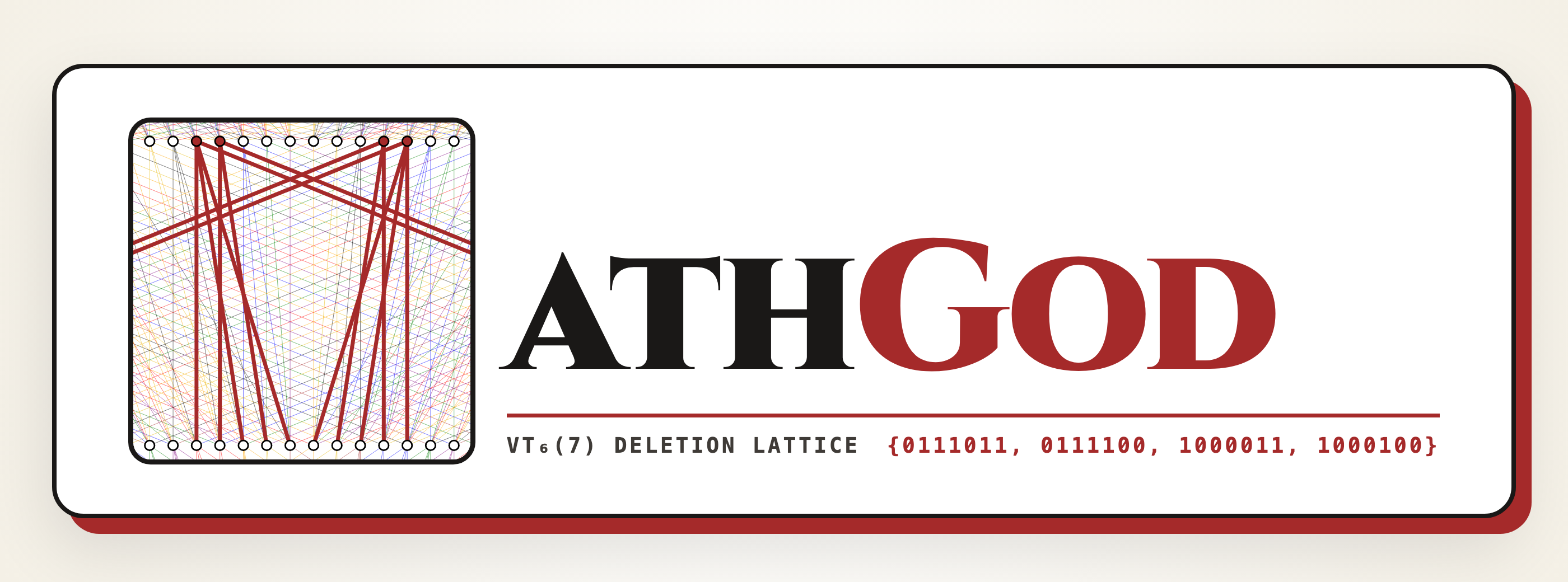
The M-athGod VT₆(7) Deletion Lattice
1965 / 2026Aesthetic & Structural

The M-athGod VT₆(7) Deletion Lattice

Bitwise-Complement Symmetry in Varshamov–Tenengolts Codes

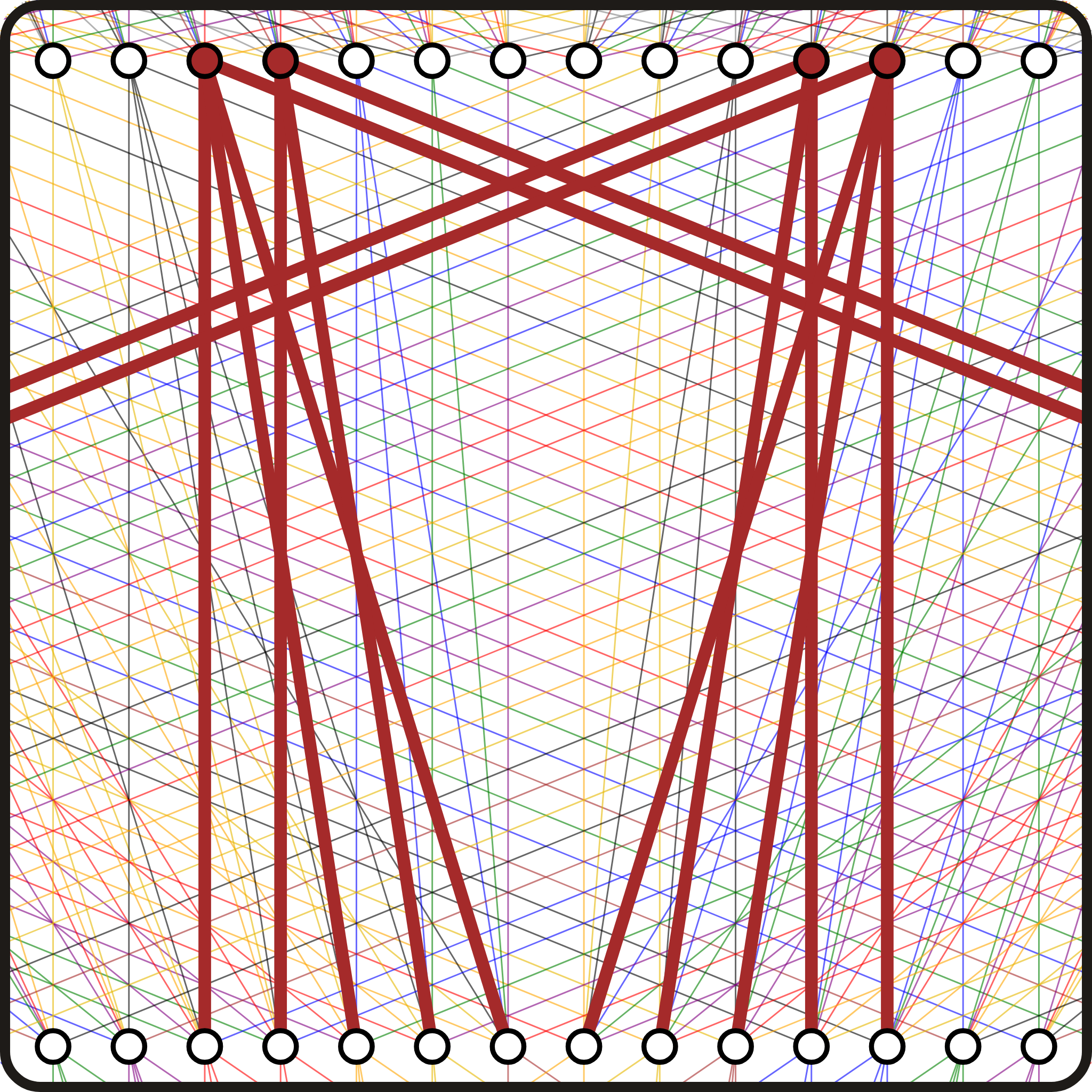
In the L=7 → L=6 Varshamov–Tenengolts single-deletion bipartite graph, the four central codewords with checksum 6 (mod 8)—0111011, 0111100, 1000011, and 1000100—are exact bitwise-complement pairs. Their 1-deletion shadows partition all 10 central nodes of {0,1}⁶ without a single collision while tracing a monumental crimson "M".

INVARIANT //∀ x ∈ {0111011, 0111100, 1000011, 1000100}, ∑ i·xᵢ ≡ 6 (mod 8) ⟹ Disjoint Deletion Spheres on {0,1}⁶

Types of Real Numbers: A Comparative Study
Radó 1962 / ConstructivismMathematical Humor

Types of Real Numbers: A Comparative Study

The Busy Beaver on ℕ vs. Irrational Constants & Non-Computable Trash

Tibor Radó’s Busy Beaver (Σ(n)) stands with wrench in hand on the clean, discrete integer ticks of the Natural Numbers (0, 1, 2, 3, 4, 5, 6), while below on the continuum ℝ, algebraic irrationals (√2, φ), transcendental constants (e, π), and Feigenbaum’s bifurcation constant (δ ≈ 4.67) pile up amidst uncomputable Borel–Chaitin trash.

INVARIANT //μ(ℚ) = 0 ∧ |ℕ| = ℵ₀ < 2^ℵ₀ = |ℝ| (Almost all real numbers are uncomputable Chaitin Ω-junk)
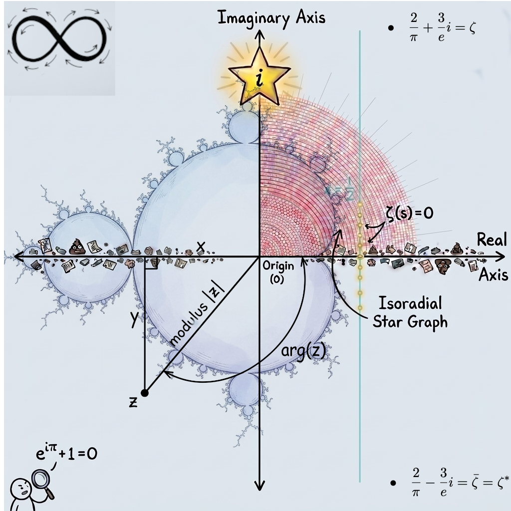
The Complex Plane, Euler’s Detective & The Critical Line
Euler 1748 • Riemann 1859Historical & Humorous

The Complex Plane, Euler’s Detective & The Critical Line

Mandelbrot Halo, Isoradial Star Graph & Non-Trivial Zeros ζ(s) = 0

A unified cartographic still of ℂ: the imaginary unit i shines as a five-pointed star atop the vertical axis, the Mandelbrot cardioid embraces the origin while irrational trash litters the real line, the Isoradial Star Graph fills Quadrant I across Riemann’s critical line Re(s) = 1/2, and in the bottom-left corner a tiny detective inspects Euler’s identity e^(iπ) + 1 = 0.

INVARIANT //e^(iπ) + 1 = 0 | ζ(s) = 0 ⟹ Re(s) = 1/2 | z = |z|·e^(i·arg(z))
The Symmetric VT₆(7) Deletion "M" Stencil
Levenshtein 1966Aesthetic & Structural

The Symmetric VT₆(7) Deletion "M" Stencil

Close-Up 1:1 Still of the Bipartite Single-Deletion Web

Pure 1:1 close-up still of the 14 central vertices of level L=7 (top row) and level L=6 (bottom row) in the Varshamov–Tenengolts deletion graph. Each background rainbow thread colors a binary string by its syndrome mod (L+1), while the 14 thick crimson edges project the four central VT₆(7) codewords onto 10 consecutive 6-bit targets.

INVARIANT //x_math(L, v) = -2^(L-1) + v, y_math(L) = L², Δy_math(7 → 6) = 49 - 36 = 13
VT-Automata Overcrowd Swarm (Zero-Deletion Explosion)
Varshamov–Tenengolts 1965 • MathGod LabAesthetic & Structural

VT-Automata Overcrowd Swarm (Zero-Deletion Explosion)

400+ Evolving Binary Codewords Linked by Single-Bit Insertion Edges in Primordial 0/1 Soup

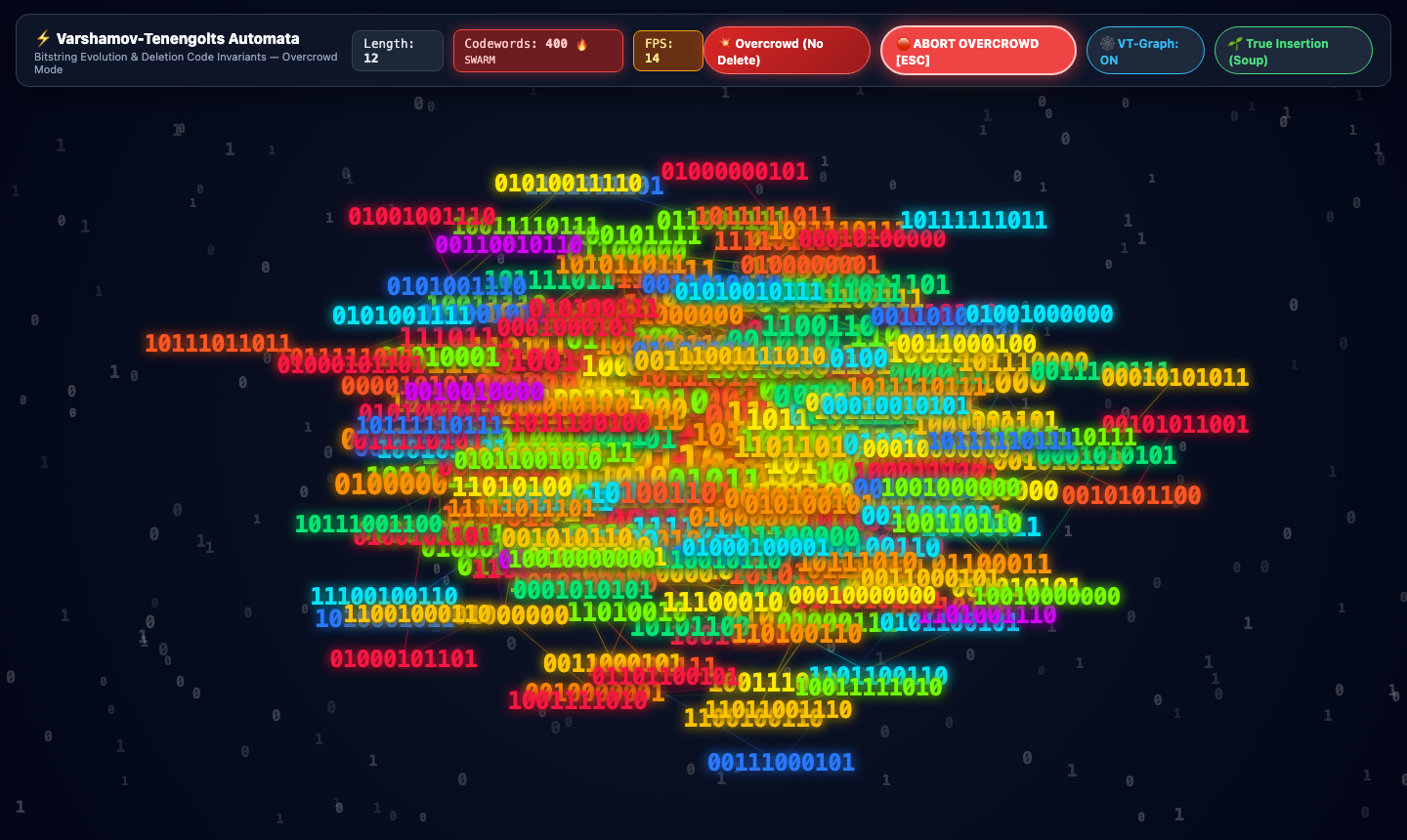
A frozen frame inside the Varshamov–Tenengolts Automata when the population cap is disengaged ("Overcrowd Mode: No Delete"). Starting from a single 0 and 1 swimming in the primordial bit soup, strings absorb drifting bits and branch into their single-insertion spheres I₁(x) up to length L = 12, coloring each codeword by its VT syndrome ∑ i·xᵢ mod (L+1) while glowing web threads link parent-child deletion pairs.

INVARIANT //y ∈ I₁(x) ⟺ x ∈ D₁(y), |I₁(x)| = L + 2, Syndrome c(x) = ∑_(i=1)^L i·xᵢ mod (L+1)
Incompressible Navier–Stokes Vortex Street & Eulerian Vector Field
Euler 1757 • Navier 1822 • Stokes 1845Aesthetic & Structural

Incompressible Navier–Stokes Vortex Street & Eulerian Vector Field

Lagrangian Streamlines, Eulerian Velocity Arrows u(x,y,t) & Live Forward-Euler Algebra Dynamo

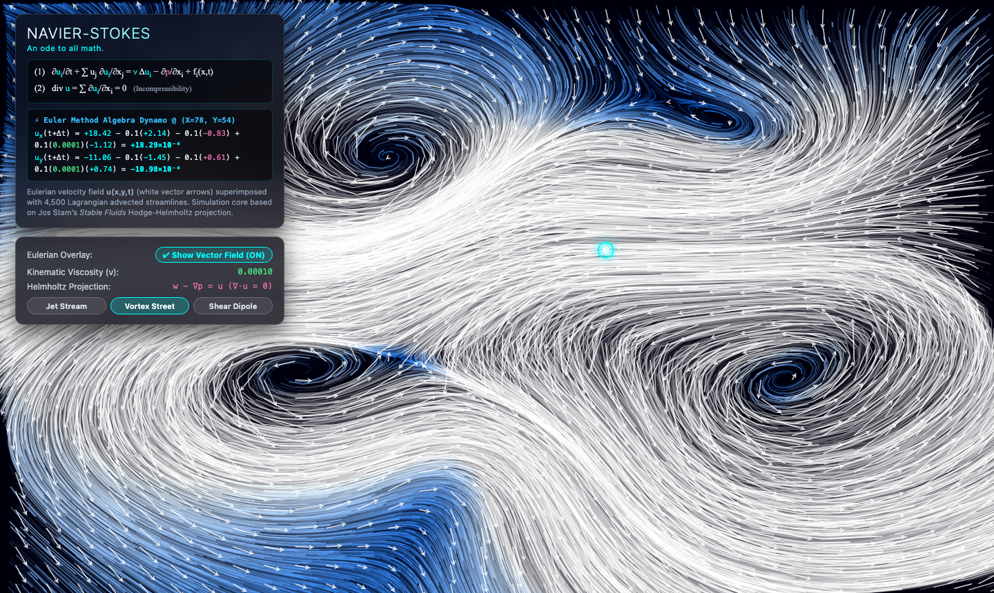
A still of 2D incompressible fluid flow with the Eulerian velocity vector field turned on: crisp white tangent arrows sample u(x,y,t) across the grid over 5,200 luminous Lagrangian particle trajectories swirling around counter-rotating Lamb–Oseen vortices, while the glowing cyan tracker particle at (X=78, Y=54) feeds live central-difference gradients into the Forward-Euler Algebra Dynamo.

INVARIANT //∂u/∂t + (u·∇)u = ν Δu − ∇p, ∇·u = 0 (Hodge–Helmholtz Projection: u = P(w) = w − ∇Δ⁻¹(∇·w))
Combinatorial Ablation of the n = 5 Deletion Code Matrix (k = 1 … 5)
Levenshtein 1966 • Combinatorial DesignHistorical & Foundational

Combinatorial Ablation of the n = 5 Deletion Code Matrix (k = 1 … 5)

Dyadic Stride-2^(k−1) Staircases, Run-Length Column Footprints & Block-Capacity Collapse

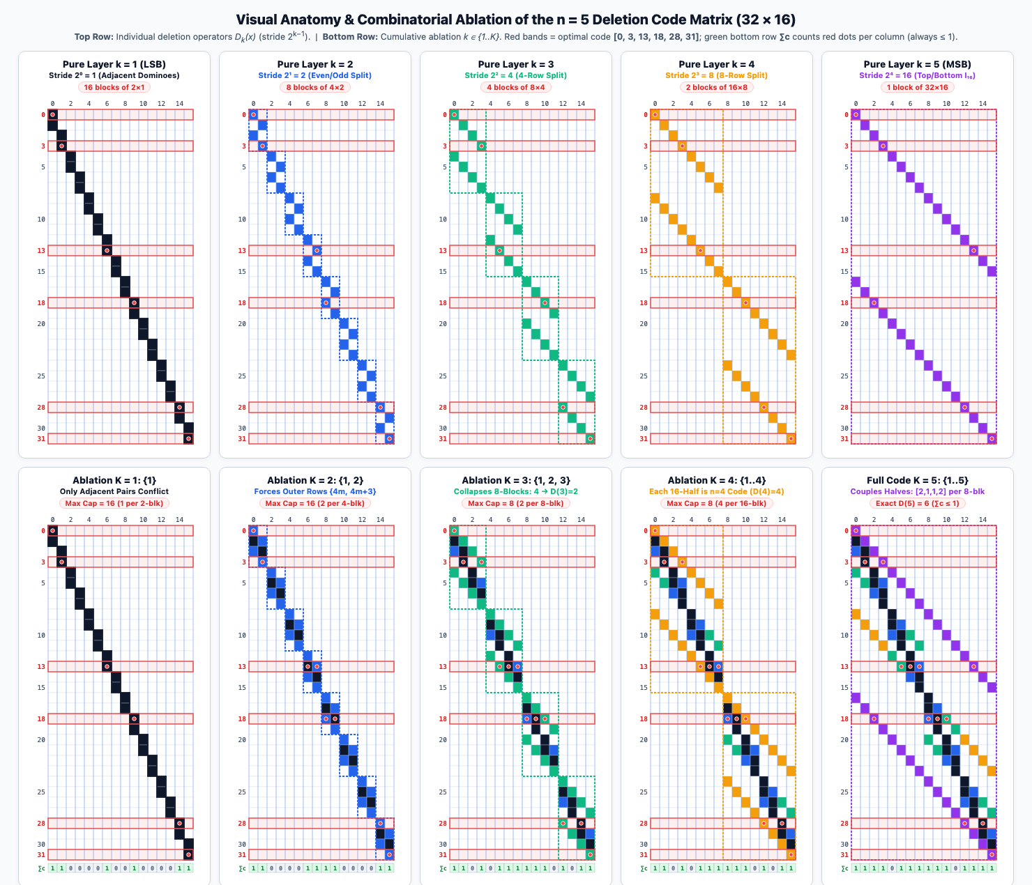
Ten-panel anatomical dissection of the 32 × 16 single-deletion incidence matrix for n = 5. The top row isolates each bit-deletion operator D_k(x) (stride 2^(k−1)); the bottom row stacks them cumulatively from K = 1 (16 adjacent 2×1 dominoes) to K = 5, showing how dyadic block capacities collapse (16 → 16 → 8 → 8 → 6) and leave the 6 red codewords [0, 3, 13, 18, 28, 31] with at most one dot per column (∑c ≤ 1).

INVARIANT //|{D₁(x), …, D_K(x)}| = runs(x[1..K]), ∀ m, |C ∩ [m·2^K, (m+1)2^K − 1]| ≤ D(K)
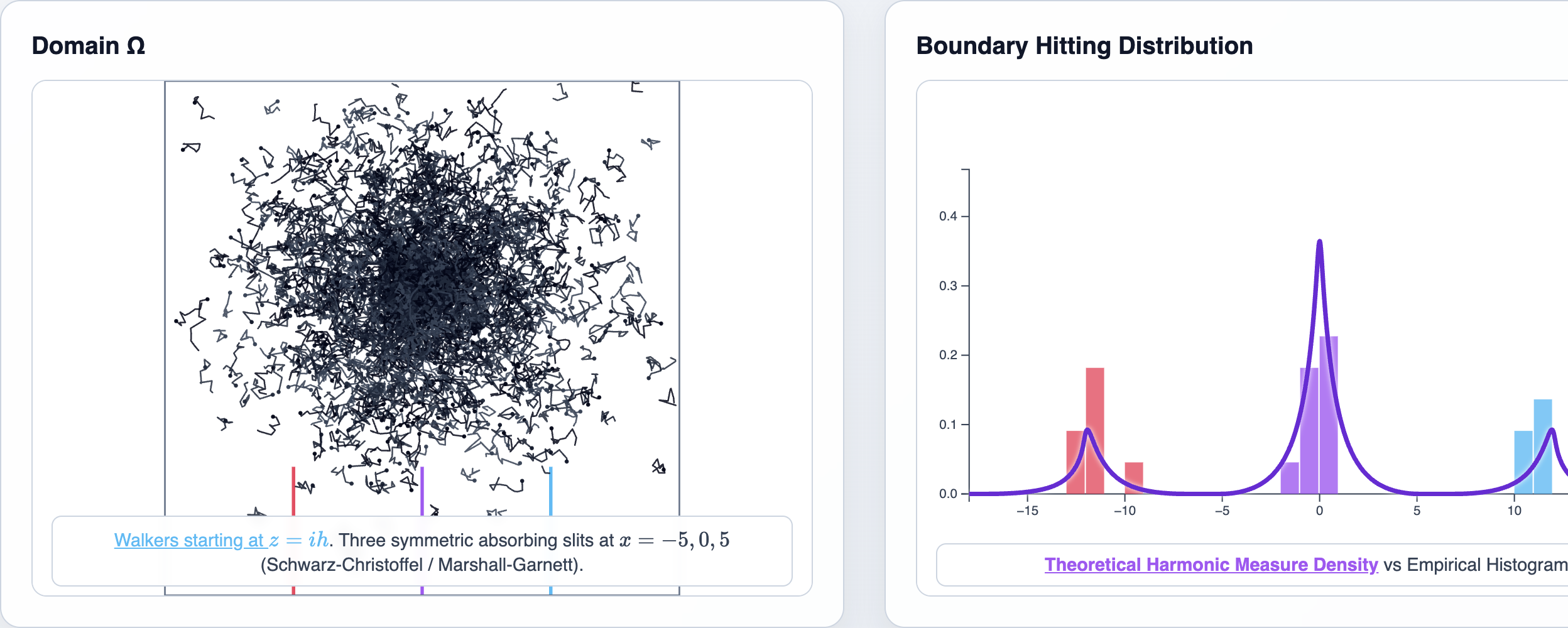
Harmonic Measure Screening on Three Symmetric Absorbing Slits
Schwarz‑Christoffel 1869 • Kakutani 1944 • Garnett & Marshall 2005Aesthetic & Structural

Harmonic Measure Screening on Three Symmetric Absorbing Slits

Schwarz‑Christoffel Slit Mapping, Marshall‑Garnett Screening & Dark-Ink Brownian Cloud (x = −5, 0, 5)

When planar dark-ink walkers descend from z = ih toward three symmetric vertical slits at x = −5 (coral), x = 0 (violet), and x = +5 (sky blue), the central slit acts as a conformal Faraday cage: it intercepts nearly 80% of all trajectories before they can diffuse into the outer fjords. Unlike half-plane or single-slit domains, mapping the upper half-plane ℍ onto a multi-slit polygon requires an irreducible Schwarz‑Christoffel integral f(ζ) = A + C ∫ ∏ (ξ − ξ_k)^(α_k − 1) dξ (whose factors cannot be separated into independent 1-slit integrals and have no elementary closed-form inverse, solved numerically via Donald E. Marshall’s Zipper / Schwarz‑Christoffel algorithms), shown as the purple theoretical density curve atop the empirical histogram.

INVARIANT //f(ζ) = A + C ∫ ∏(ξ − τ_k)¹(ξ − β_j)^(−1/2) dξ, ω(ih, S₀) ≫ ω(ih, S±₁) (Schwarz‑Christoffel & Garnett‑Marshall Harmonic Measure)
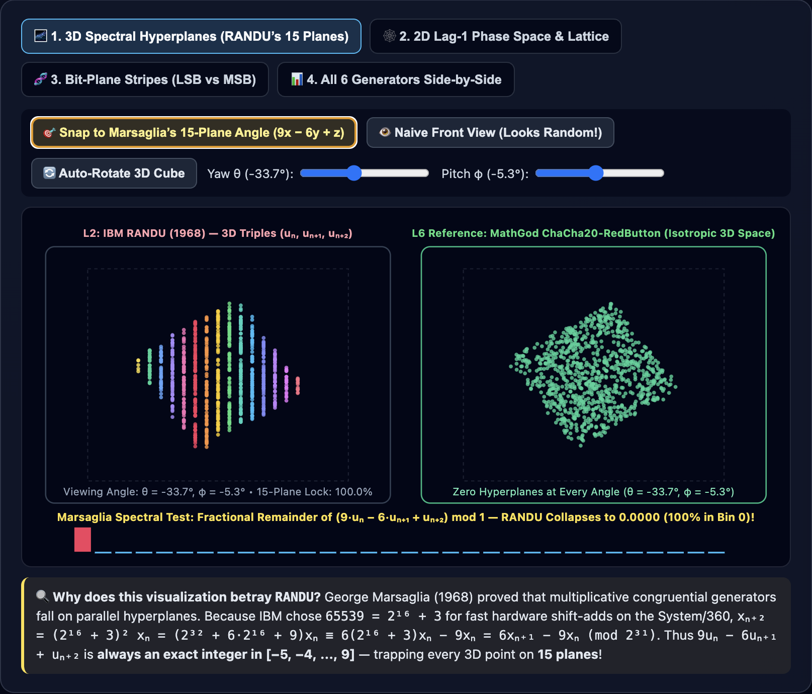
Why IBM RANDU (1968) Failed the 3D Spectral Lattice Test
Marsaglia 1968 • ChaCha20 / RFC 8439Historical & Foundational

Why IBM RANDU (1968) Failed the 3D Spectral Lattice Test

Marsaglia’s 15 Parallel Hyperplanes (9x − 6y + z ≡ 0 mod 2³¹) vs. Isotropic ChaCha20-RedButton

For decades, IBM’s Scientific Subroutine Package shipped RANDU (x_{n+1} = 65539·x_n mod 2³¹) because 65539 = 2¹⁶ + 3 was fast in hardware. In 1D and 2D it looks like uniform white noise—but rotating the 3D delay triple (u_n, u_{n+1}, u_{n+2}) to the normal vector n = (9, −6, 1) reveals that every point in ℝ³ is trapped on just 15 parallel planes, whereas our nanosecond-seeded ChaCha20 stream fills the cube isotropically.

INVARIANT //65539² ≡ 6·65539 − 9 (mod 2³¹) ⟹ x_{n+2} − 6x_{n+1} + 9x_n ≡ 0 (mod 2³¹) (15 Marsaglia Planes)